雀悅 - 恢復自由了

5月 03 週一 201014:57
HOW TO：以透明度繪製影像

http://msdn.microsoft.com/zh-tw/library/ms172507(VS.80).aspx.NET Compact Framework 支援透明度，但只有一種透明度色彩。SetColorKey 方法必須針對低色彩和高色彩範圍指定相同的色彩。此範例會以紅色和黑色的設計來建立矩形的 Bitmap，並示範兩種設定透明度的技巧：根據影像的像素來使用 SetColorKey 方法。此範例會使用影像左上方的像素來設定透明度。因為此像素是黑色的，所有原先為黑色的像素將會變成透明。

以明確的色彩設定來使用 SetColorKey 方法。此範例會將色彩設為紅色，因此所有原先為紅色的像素將會變成透明。

若要示範，先將兩種透明度技巧標記為註解再執行應用程式，以查看影像沒有設定透明度時出現的樣子。然後針對其中一種技巧，取消註解程式碼。

// The .NET Compact Framework supports transparency,

// but with only one transparency color.

// The SetColorKey method must have the same color

// specified for the low color and high color range.

 // Note that you must uncomment lines of code

// as indicated for the desired transparency effect.

protected override void OnPaint(PaintEventArgs e) {

// Create a red and black bitmap to demonstrate transparency.

Bitmap bmp = new Bitmap(75,75);

Graphics g = Graphics.FromImage(bmp);

g.FillEllipse(new SolidBrush(Color.Red), 0, 0, bmp.Width, bmp.Width);

g.DrawLine(new Pen(Color.Black), 0, 0, bmp.Width, bmp.Width);

g.DrawLine(new Pen(Color.Black), bmp.Width, 0, 0, bmp.Width);

g.Dispose(); ImageAttributes attr = new ImageAttributes();

// Set the transparency color key based on the upper-left pixel

// of the image.

// Uncomment the following line to make all black pixels transparent:

// attr.SetColorKey(bmp.GetPixel(0, 0), bmp.GetPixel(0, 0));

 // Set the transparency color key based on a specified value.

// Uncomment the following line to make all red pixels transparent:

// attr.SetColorKey(Color.Red, Color.Red);

// Draw the image using the image attributes.

Rectangle dstRect = new Rectangle(0, 0, bmp.Width, bmp.Height);

e.Graphics.DrawImage(bmp, dstRect, 0, 0, bmp.Width, bmp.Height,GraphicsUnit.Pixel, attr);

(繼續閱讀...)

雀悦發表在痞客邦留言(0) 人氣(20)

個人分類：image processing

▲top

5月 03 週一 201014:57
HOW TO：以透明度繪製影像

http://msdn.microsoft.com/zh-tw/library/ms172507(VS.80).aspx.NET Compact Framework 支援透明度，但只有一種透明度色彩。SetColorKey 方法必須針對低色彩和高色彩範圍指定相同的色彩。此範例會以紅色和黑色的設計來建立矩形的 Bitmap，並示範兩種設定透明度的技巧：根據影像的像素來使用 SetColorKey 方法。此範例會使用影像左上方的像素來設定透明度。因為此像素是黑色的，所有原先為黑色的像素將會變成透明。

以明確的色彩設定來使用 SetColorKey 方法。此範例會將色彩設為紅色，因此所有原先為紅色的像素將會變成透明。

若要示範，先將兩種透明度技巧標記為註解再執行應用程式，以查看影像沒有設定透明度時出現的樣子。然後針對其中一種技巧，取消註解程式碼。

// The .NET Compact Framework supports transparency,

// but with only one transparency color.

// The SetColorKey method must have the same color

// specified for the low color and high color range.

 // Note that you must uncomment lines of code

// as indicated for the desired transparency effect.

protected override void OnPaint(PaintEventArgs e) {

// Create a red and black bitmap to demonstrate transparency.

Bitmap bmp = new Bitmap(75,75);

Graphics g = Graphics.FromImage(bmp);

g.FillEllipse(new SolidBrush(Color.Red), 0, 0, bmp.Width, bmp.Width);

g.DrawLine(new Pen(Color.Black), 0, 0, bmp.Width, bmp.Width);

g.DrawLine(new Pen(Color.Black), bmp.Width, 0, 0, bmp.Width);

g.Dispose(); ImageAttributes attr = new ImageAttributes();

// Set the transparency color key based on the upper-left pixel

// of the image.

// Uncomment the following line to make all black pixels transparent:

// attr.SetColorKey(bmp.GetPixel(0, 0), bmp.GetPixel(0, 0));

 // Set the transparency color key based on a specified value.

// Uncomment the following line to make all red pixels transparent:

// attr.SetColorKey(Color.Red, Color.Red);

// Draw the image using the image attributes.

Rectangle dstRect = new Rectangle(0, 0, bmp.Width, bmp.Height);

e.Graphics.DrawImage(bmp, dstRect, 0, 0, bmp.Width, bmp.Height,GraphicsUnit.Pixel, attr);

(繼續閱讀...)

雀悦發表在痞客邦留言(0) 人氣(43)

個人分類：image processing

▲top

5月 03 週一 201014:55
c#如何调整图片透明度

http://bbs.techrepublic.com.cn/thread-792692-1-1.html
对图片的透明度的调整可以通过重绘并且对颜色进行调整得到实现
C#中对颜色的调整是通过一个ColorMatrix的对象实现的这个对象表示一个5X5的矩阵用于对颜色进行线性的变换作为一般的理解只需要指定一个如下的矩阵即可实现对颜色的变换：
1，0，0，0，0
0，1，0，0，0
0，0，1，0，0
0，0，0，透明度,0
0，0，0，0，1
简单的代码如下：
//注意using System.Drawing名字空间 opacity是想要设定的透明度
float[][] nArray ={ new float[] {1, 0, 0, 0, 0},
new float[] {0, 1, 0, 0, 0},
new float[] {0, 0, 1, 0, 0},
new float[] {0, 0, 0, opacity, 0},
new float[] {0, 0, 0, 0, 1}};
ColorMatrix matrix = new ColorMatrix(nArray);
ImageAttributes attributes = new ImageAttributes();
attributes.SetColorMatrix(matrix, ColorMatrixFlag.Default, ColorAdjustType.Bitmap )
Image srcImage = Image.FromFile("aaa.jpg");
Bitmap resultImage = new Bitmap(srcImage.Width, srcImage.Height);
Graphics g = Graphics.FromImage(resultImage);
g.DrawImage( srcImage, new Rectangle( 0, 0, srcImage.Width, srcImage.Height ), 0, 0, srcImage.Width, srcImage.Height, GraphicsUnit.Pixel, attributes);
//resultImage就是楼主想要的结果了

(繼續閱讀...)

雀悦發表在痞客邦留言(0) 人氣(976)

個人分類：image processing

▲top

5月 03 週一 201014:55
c#如何调整图片透明度

http://bbs.techrepublic.com.cn/thread-792692-1-1.html
对图片的透明度的调整可以通过重绘并且对颜色进行调整得到实现
C#中对颜色的调整是通过一个ColorMatrix的对象实现的这个对象表示一个5X5的矩阵用于对颜色进行线性的变换作为一般的理解只需要指定一个如下的矩阵即可实现对颜色的变换：
1，0，0，0，0
0，1，0，0，0
0，0，1，0，0
0，0，0，透明度,0
0，0，0，0，1
简单的代码如下：
//注意using System.Drawing名字空间 opacity是想要设定的透明度
float[][] nArray ={ new float[] {1, 0, 0, 0, 0},
new float[] {0, 1, 0, 0, 0},
new float[] {0, 0, 1, 0, 0},
new float[] {0, 0, 0, opacity, 0},
new float[] {0, 0, 0, 0, 1}};
ColorMatrix matrix = new ColorMatrix(nArray);
ImageAttributes attributes = new ImageAttributes();
attributes.SetColorMatrix(matrix, ColorMatrixFlag.Default, ColorAdjustType.Bitmap )
Image srcImage = Image.FromFile("aaa.jpg");
Bitmap resultImage = new Bitmap(srcImage.Width, srcImage.Height);
Graphics g = Graphics.FromImage(resultImage);
g.DrawImage( srcImage, new Rectangle( 0, 0, srcImage.Width, srcImage.Height ), 0, 0, srcImage.Width, srcImage.Height, GraphicsUnit.Pixel, attributes);
//resultImage就是楼主想要的结果了

(繼續閱讀...)

雀悦發表在痞客邦留言(0) 人氣(130)

個人分類：image processing

▲top

2月 09 週二 201017:04
Sobel Filter

http://140.134.32.129/oe/oe/lcd/subject4-3.htm
Sobel Filter
對於一個二值化後的影像，要尋找影像的邊緣最常見的就是使用Sobel Filter，這個運算包含兩個運算子如下：
(2.1)

(繼續閱讀...)

雀悦發表在痞客邦留言(0) 人氣(58)

個人分類：image processing

▲top

2月 09 週二 201017:04
Sobel Filter

http://140.134.32.129/oe/oe/lcd/subject4-3.htm
Sobel Filter
對於一個二值化後的影像，要尋找影像的邊緣最常見的就是使用Sobel Filter，這個運算包含兩個運算子如下：
(2.1)

(繼續閱讀...)

雀悦發表在痞客邦留言(0) 人氣(125)

個人分類：image processing

▲top

2月 02 週二 201016:24
常用图形学名词解释

http://www.cnblogs.com/Lhw978/archive/2009/11/30/1614052.html

(繼續閱讀...)

雀悦發表在痞客邦留言(0) 人氣(1)

個人分類：image processing

▲top

2月 02 週二 201016:24
常用图形学名词解释

http://www.cnblogs.com/Lhw978/archive/2009/11/30/1614052.html

(繼續閱讀...)

雀悦發表在痞客邦留言(0) 人氣(4)

個人分類：image processing

▲top

2月 02 週二 201015:00
Color correction matrix

http://www.imatest.com/docs/colormatrix.html

Introduction

Multicharts can calculate a color correction matrix that can be applied to images to achieve optimum color balance, as defined by minimizing a color error parameter on the test chart of choice. (The default is the mean of (Delta-E 94)² for all patches where L*>10 and L*<95.)>

Some of the background for the calculation can be found in Color Correction Matrix for Digital Still and Video Imaging Systems by Stephen Wolf, though the Imatest calculation differs in many respects: there is no issue with outliers and optimization is performed using one of the standard color difference metrics.

The color correction matrix is initially included only in Multicharts.

The Math

The matrix

Color images are stored in m x n x 3 arrays (m rows (height) x n columns (width) x 3 colors). For the sake of simplicity, we transform the color image to a k x 3 array, where k = m x n. An Original (uncorrected) array O can be represented as

 | O_R1 O_G1 O_B1 | O = | O_R2 O_G2 O_B2 | | ... |
| ... |
| O_Rk O_Gk O_Bk |

where O_Ri, O_Gi, and O_Bi represent the normalized R, G, and B levels of pixel i. The transformed (corrected) array is calledP, where

P = O A (case 1: A is a 3x3 matrix) — or —
P = [O 1] A (case 2: A is a 4x3 matrix; the added column of 1s provides a dc-offset)

A is the 3x3 or 4x3 color correction matrix. For the 3x3 matrix (case 1),

 | P_R1 P_G1 P_B1 | | O_R1 O_G1 O_B1 | P = | P_R2 P_G2 P_B2 | = | O_R2 O_G2 O_B2 | | A11 A12 A13 | | ... | | ... | X | A21 A22 A23 |
| ... | | ... | | A31 A32 A33 |
| P_Rk P_Gk P_Bk | | O_Rk O_Gk O_Bk |

X denotes matrix multiplication. In this case, for row m,

P_Rm = O_Rm*A11 + O_Gm*A21 + O_Bm*A31 (* denotes multiplication.)
P_Gm = O_Rm*A12 + O_Gm*A22 + O_Bm*A32
P_Bm = O_Rm*A13 + O_Gm*A23 + O_Bm*A33

For the 4x3 matrix (case 2), a column of 1s is added to provide a dc-offset,

 | P_R1 P_G1 P_B1 | | O_R1 O_G1 O_B1 1 | | A11 A12 A13 | P = | P_R2 P_G2 P_B2 | = | O_R2 O_G2 O_B2 1 | | A21 A22 A23 | | ... | | ... | X | A31 A32 A33 |
| ... | | ... | | A41 A42 A43 |
| P_Rk P_Gk P_Bk | | O_Rk O_Gk O_Bk 1 |

In this case, for row m,

P_Rm = O_Rm*A11 + O_Gm*A21 + O_Bm*A31 + A41
P_Gm = O_Rm*A12 + O_Gm*A22 + O_Bm*A32 + A42
P_Bm = O_Rm*A13 + O_Gm*A23 + O_Bm*A33 + A43

The goal of the calculation is to minimize the difference (the mean square error metric) between P and the reference array (the ideal chart values) R. The initial values of A (the starting point for optimization) for the 3x3 and 4x3 cases, are

 | k_R 0 0 | | k_R 0 0 | A(3x3) = | 0 k_G 0 | ; A(4x3) = | 0 k_G 0 | | 0 0 k_B | | 0 0 k_B |
| 0 0 0 |

where

k_R = mean(R_Ri ; all i) ⁄ mean(O_Ri ; all i) for reference array R and original array O
k_G = mean(R_Gi ; all i) ⁄ mean(O_Gi ; all i)
k_B = mean(R_Bi ; all i) ⁄ mean(O_Bi ; all i)

These starting values are closer to the final values (have less mean square error) than the identity matrix (k_R = k_G = k_B = 1). They tend to converge slightly better.

Linearization

Although most digital image sensors are linear up to the point where they saturate, image files are highly nonlinear— they are designed for display at a specified gamma ( γ ), where display luminance = pixel level^γ. Gamma = 2.2 for the most commonly used color spaces (sRGB, Adobe RGB (1998) and Wide Gamut RGB (WGRGB)), although some well-known color spaces are designed for display at gamma = 1.8 (ProPhoto, Apply, ColorMatch; all RGB).

When cameras encode images (a part of the RAW conversion process), they apply a gamma that is the approximate inverse of the display gamma. Perhaps we should say very approximate: it may vary considerably from 1/γ, and it often includes a tonal response curve "shoulder" (an area of reduced contrast) to minimize highlight burnout. The shoulder makes the response more "film-like," improving pictorial quality in most instances.

If the input image is gamma-encoded you may wish to linearize the image prior to applying the correction matrix. Imatest has several linearization options.

Optimization steps

(Optionally) linearize the input image. If Color space gamma linearization is selected, O_L = O^γ.
Call the optimizer, which
- calculates a (temporary) corrected image T_L = O_L A.
- (Optionally) removes the linearization: T = T_L^(1/γ)
- Finds the mean of squares of errors between T and the reference (ideal) array R. The error is one of the standard error measurements: ΔE*_ab, ΔC*_ab, ΔE₉₄, ΔE₉₄, ΔE_CMC, ΔC_CMC, ΔE₀₀, or ΔC₀₀, described here. ΔE₉₄ is the recommended default. Although the CIEDE2000 color error metrics (ΔE₀₀, ...) are more accurate, they contain small discontinuities that can affect optimization, and hence they should be used with caution. SeeSharma for details. The ΔC errors are similar to ΔE with luminance (L*) omitted.
- Adjusts A until a minimum value of the sum of squares of the errors is found, using nonlinear optimization.
- Report the final value of A.

In applying A (generally outside of Imatest), a similar linearization should be used. A may be applied during the RAW conversion process, prior to the application of the gamma + tonal response curve.

There is no guarantee that A is a global minimum. Its final value depends to some extent on its starting value.

The Color correction matrix in Multicharts

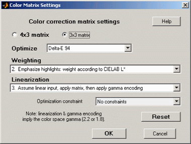
Options: Color matrix calculation options can be set by clickingSettings, Color matrix in the Multicharts window. This brings up the dialog box shown on the right. The options are

4x3 or 3x3 matrix: Color correction matrix size. The 4x3 matrix (the default) includes a dc-offset (constant) term. It may be slightly more accurate, but it takes more computation time.
Optimize: Select the color error parameter whose mean of squares over patches with L*>10 (nearly black for <10;>95) is to be minimized. Choices include ΔE ab, ΔC ab, ΔE 94, ΔE 94, ΔE CMC, ΔC CMC, ΔE 00, and ΔC 00, described here. ΔE 94 is the default value, recommended because it gives less weight to chroma differences between highly chromatic (saturated; large a*² + b*²) colors, which is closer to the eye's perception than ΔE ab (the standard ΔE value: the geometrical distance between colors in L*a*b* space).
Weighting: Set the weighting of the patches for optimization. Choices:
- 1. Equal weighting [default] Patches are equally weighted. May not be the optimum setting because highlight colors may be more visually prominent than shadow colors.
- 2. Emphasize highlights: weight according to CIELAB L* Give more weight to visually-prominent hightlight patches.
- 3. Strongly emphasize highlights: weight according to L*^2.
Linearization: Choose the method of linearizing the image (or leave it unchanged). For linearization or gamma encoding, the value of gamma ( γ ) for the selected color space (sRGB, Adobe RGB, etc.) is used. The equation for linearization isO_L = O^1/γ. The equation for gamma application O = O_L^γ.
- 1. Linearize input, apply matrix, then apply gamma encoding. Usually the best choice for images encoded in a standard color space.
- 2. No linearization: apply matrix to input pixels. May not be the best choice for gamma-encoded images, but useful for experimentation and for images that start and remain linear.
- 3. Assume linear input, apply matrix, then apply gamma encoding. A good choice for images that are not gamma-encoded, but need to be converted into a color space. Color space gamma is not applied in converting the input RGB image to L*a*b*.
- 4. Assume linear input & output (gamma = 1 throughout). No linearization or gamma encoding. Color space gamma is not applied in converting between RGB and L*a*b* spaces.
Optimization constraint
- No constraints. This is the default and should only be changed with good reason.
- Rows sum to 1.
- Columns sum to 1.

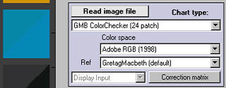
To calculate the color correction matrix, read the image into Multicharts, then press the Correction matrix button, shown on the right. The display will change, as shown below. The improvement for this image, which is quite good to begin with, is undramatic.

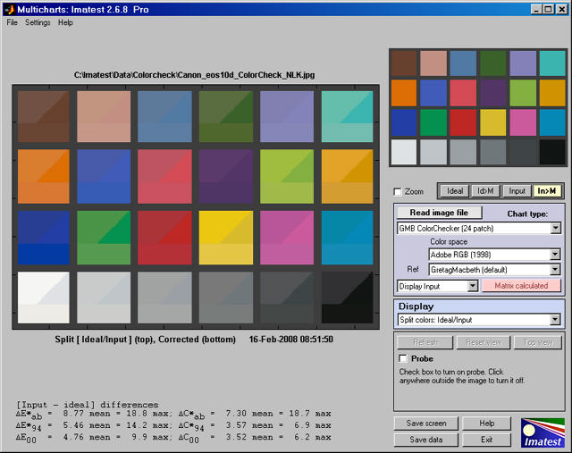
Multicharts window: split view, corrected
Split view, showing reference, input, and corrected patch colors

The image now shows the corrected colors on the bottom of each patch. The ideal (reference) color remains in the upper-left and the input (original) color remains in the upper right.

The Correction matrix button changes to Matrix calculated, highlighted with a pink background. The correction matrix cannot be recalculated until an image property changes (new image, color space, reference file, or color matrix setting). The Display input(or Corrected) dropdown menu, immediately to its left, is enabled. You can choose one of two selections.

Display input	Color differences (input − ideal) are shown in most displays, and [Input − ideal] Color differences are shown in the text in the lower left. Two displays are unaffected by this setting: Pseudocolor color difference and Split colors, where (corrected − ideal) is shown on the bottom.
Display corrected	Color differences (corrected − ideal) are shown in most displays, and [Corrected − ideal] Color differences are shown in the text in the lower left.

The EXIF data and Color matrix display has a summary of results.

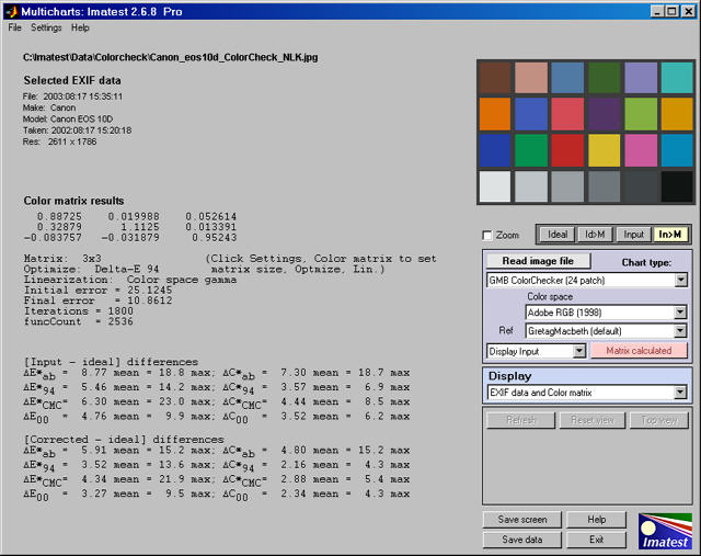
Exif data and color correction summary
Exif and Color matrix view

The color correct matrix, results summary, and both [input - ideal] and [corrected -ideal] color difference summaries are shown. The initial and final error numbers shows how much the selected metric (in this case the sum of squares of Delta-E 94 for all patches with L*>10 and L*<95)>

(繼續閱讀...)

雀悦發表在痞客邦留言(0) 人氣(1,292)

個人分類：image processing

▲top

2月 02 週二 201015:00
Color correction matrix

http://www.imatest.com/docs/colormatrix.html

Introduction

Multicharts can calculate a color correction matrix that can be applied to images to achieve optimum color balance, as defined by minimizing a color error parameter on the test chart of choice. (The default is the mean of (Delta-E 94)² for all patches where L*>10 and L*<95.)>

Some of the background for the calculation can be found in Color Correction Matrix for Digital Still and Video Imaging Systems by Stephen Wolf, though the Imatest calculation differs in many respects: there is no issue with outliers and optimization is performed using one of the standard color difference metrics.

The color correction matrix is initially included only in Multicharts.

The Math

The matrix

Color images are stored in m x n x 3 arrays (m rows (height) x n columns (width) x 3 colors). For the sake of simplicity, we transform the color image to a k x 3 array, where k = m x n. An Original (uncorrected) array O can be represented as

 | O_R1 O_G1 O_B1 | O = | O_R2 O_G2 O_B2 | | ... |
| ... |
| O_Rk O_Gk O_Bk |

where O_Ri, O_Gi, and O_Bi represent the normalized R, G, and B levels of pixel i. The transformed (corrected) array is calledP, where

P = O A (case 1: A is a 3x3 matrix) — or —
P = [O 1] A (case 2: A is a 4x3 matrix; the added column of 1s provides a dc-offset)

A is the 3x3 or 4x3 color correction matrix. For the 3x3 matrix (case 1),

 | P_R1 P_G1 P_B1 | | O_R1 O_G1 O_B1 | P = | P_R2 P_G2 P_B2 | = | O_R2 O_G2 O_B2 | | A11 A12 A13 | | ... | | ... | X | A21 A22 A23 |
| ... | | ... | | A31 A32 A33 |
| P_Rk P_Gk P_Bk | | O_Rk O_Gk O_Bk |

X denotes matrix multiplication. In this case, for row m,

P_Rm = O_Rm*A11 + O_Gm*A21 + O_Bm*A31 (* denotes multiplication.)
P_Gm = O_Rm*A12 + O_Gm*A22 + O_Bm*A32
P_Bm = O_Rm*A13 + O_Gm*A23 + O_Bm*A33

For the 4x3 matrix (case 2), a column of 1s is added to provide a dc-offset,

 | P_R1 P_G1 P_B1 | | O_R1 O_G1 O_B1 1 | | A11 A12 A13 | P = | P_R2 P_G2 P_B2 | = | O_R2 O_G2 O_B2 1 | | A21 A22 A23 | | ... | | ... | X | A31 A32 A33 |
| ... | | ... | | A41 A42 A43 |
| P_Rk P_Gk P_Bk | | O_Rk O_Gk O_Bk 1 |

In this case, for row m,

P_Rm = O_Rm*A11 + O_Gm*A21 + O_Bm*A31 + A41
P_Gm = O_Rm*A12 + O_Gm*A22 + O_Bm*A32 + A42
P_Bm = O_Rm*A13 + O_Gm*A23 + O_Bm*A33 + A43

The goal of the calculation is to minimize the difference (the mean square error metric) between P and the reference array (the ideal chart values) R. The initial values of A (the starting point for optimization) for the 3x3 and 4x3 cases, are

 | k_R 0 0 | | k_R 0 0 | A(3x3) = | 0 k_G 0 | ; A(4x3) = | 0 k_G 0 | | 0 0 k_B | | 0 0 k_B |
| 0 0 0 |

where

k_R = mean(R_Ri ; all i) ⁄ mean(O_Ri ; all i) for reference array R and original array O
k_G = mean(R_Gi ; all i) ⁄ mean(O_Gi ; all i)
k_B = mean(R_Bi ; all i) ⁄ mean(O_Bi ; all i)

These starting values are closer to the final values (have less mean square error) than the identity matrix (k_R = k_G = k_B = 1). They tend to converge slightly better.

Linearization

Although most digital image sensors are linear up to the point where they saturate, image files are highly nonlinear— they are designed for display at a specified gamma ( γ ), where display luminance = pixel level^γ. Gamma = 2.2 for the most commonly used color spaces (sRGB, Adobe RGB (1998) and Wide Gamut RGB (WGRGB)), although some well-known color spaces are designed for display at gamma = 1.8 (ProPhoto, Apply, ColorMatch; all RGB).

When cameras encode images (a part of the RAW conversion process), they apply a gamma that is the approximate inverse of the display gamma. Perhaps we should say very approximate: it may vary considerably from 1/γ, and it often includes a tonal response curve "shoulder" (an area of reduced contrast) to minimize highlight burnout. The shoulder makes the response more "film-like," improving pictorial quality in most instances.

If the input image is gamma-encoded you may wish to linearize the image prior to applying the correction matrix. Imatest has several linearization options.

Optimization steps

(Optionally) linearize the input image. If Color space gamma linearization is selected, O_L = O^γ.
Call the optimizer, which
- calculates a (temporary) corrected image T_L = O_L A.
- (Optionally) removes the linearization: T = T_L^(1/γ)
- Finds the mean of squares of errors between T and the reference (ideal) array R. The error is one of the standard error measurements: ΔE*_ab, ΔC*_ab, ΔE₉₄, ΔE₉₄, ΔE_CMC, ΔC_CMC, ΔE₀₀, or ΔC₀₀, described here. ΔE₉₄ is the recommended default. Although the CIEDE2000 color error metrics (ΔE₀₀, ...) are more accurate, they contain small discontinuities that can affect optimization, and hence they should be used with caution. SeeSharma for details. The ΔC errors are similar to ΔE with luminance (L*) omitted.
- Adjusts A until a minimum value of the sum of squares of the errors is found, using nonlinear optimization.
- Report the final value of A.

In applying A (generally outside of Imatest), a similar linearization should be used. A may be applied during the RAW conversion process, prior to the application of the gamma + tonal response curve.

There is no guarantee that A is a global minimum. Its final value depends to some extent on its starting value.

The Color correction matrix in Multicharts

Options: Color matrix calculation options can be set by clickingSettings, Color matrix in the Multicharts window. This brings up the dialog box shown on the right. The options are

4x3 or 3x3 matrix: Color correction matrix size. The 4x3 matrix (the default) includes a dc-offset (constant) term. It may be slightly more accurate, but it takes more computation time.
Optimize: Select the color error parameter whose mean of squares over patches with L*>10 (nearly black for <10;>95) is to be minimized. Choices include ΔE ab, ΔC ab, ΔE 94, ΔE 94, ΔE CMC, ΔC CMC, ΔE 00, and ΔC 00, described here. ΔE 94 is the default value, recommended because it gives less weight to chroma differences between highly chromatic (saturated; large a*² + b*²) colors, which is closer to the eye's perception than ΔE ab (the standard ΔE value: the geometrical distance between colors in L*a*b* space).
Weighting: Set the weighting of the patches for optimization. Choices:
- 1. Equal weighting [default] Patches are equally weighted. May not be the optimum setting because highlight colors may be more visually prominent than shadow colors.
- 2. Emphasize highlights: weight according to CIELAB L* Give more weight to visually-prominent hightlight patches.
- 3. Strongly emphasize highlights: weight according to L*^2.
Linearization: Choose the method of linearizing the image (or leave it unchanged). For linearization or gamma encoding, the value of gamma ( γ ) for the selected color space (sRGB, Adobe RGB, etc.) is used. The equation for linearization isO_L = O^1/γ. The equation for gamma application O = O_L^γ.
- 1. Linearize input, apply matrix, then apply gamma encoding. Usually the best choice for images encoded in a standard color space.
- 2. No linearization: apply matrix to input pixels. May not be the best choice for gamma-encoded images, but useful for experimentation and for images that start and remain linear.
- 3. Assume linear input, apply matrix, then apply gamma encoding. A good choice for images that are not gamma-encoded, but need to be converted into a color space. Color space gamma is not applied in converting the input RGB image to L*a*b*.
- 4. Assume linear input & output (gamma = 1 throughout). No linearization or gamma encoding. Color space gamma is not applied in converting between RGB and L*a*b* spaces.
Optimization constraint
- No constraints. This is the default and should only be changed with good reason.
- Rows sum to 1.
- Columns sum to 1.

To calculate the color correction matrix, read the image into Multicharts, then press the Correction matrix button, shown on the right. The display will change, as shown below. The improvement for this image, which is quite good to begin with, is undramatic.

Multicharts window: split view, corrected
Split view, showing reference, input, and corrected patch colors

The image now shows the corrected colors on the bottom of each patch. The ideal (reference) color remains in the upper-left and the input (original) color remains in the upper right.

The Correction matrix button changes to Matrix calculated, highlighted with a pink background. The correction matrix cannot be recalculated until an image property changes (new image, color space, reference file, or color matrix setting). The Display input(or Corrected) dropdown menu, immediately to its left, is enabled. You can choose one of two selections.

Display input	Color differences (input − ideal) are shown in most displays, and [Input − ideal] Color differences are shown in the text in the lower left. Two displays are unaffected by this setting: Pseudocolor color difference and Split colors, where (corrected − ideal) is shown on the bottom.
Display corrected	Color differences (corrected − ideal) are shown in most displays, and [Corrected − ideal] Color differences are shown in the text in the lower left.

The EXIF data and Color matrix display has a summary of results.

Exif data and color correction summary
Exif and Color matrix view

The color correct matrix, results summary, and both [input - ideal] and [corrected -ideal] color difference summaries are shown. The initial and final error numbers shows how much the selected metric (in this case the sum of squares of Delta-E 94 for all patches with L*>10 and L*<95)>

(繼續閱讀...)

雀悦發表在痞客邦留言(0) 人氣(274)

個人分類：image processing

▲top

雀悅 - 恢復自由了

歡迎光臨雀悅的在痞客邦的小天地

HOW TO：以透明度繪製影像

HOW TO：以透明度繪製影像

c#如何调整图片透明度

c#如何调整图片透明度

Sobel Filter

Sobel Filter

常用图形学名词解释

常用图形学名词解释

Color correction matrix

Introduction

The Math

The matrix

Linearization

Optimization steps

The Color correction matrix in Multicharts

Color correction matrix

Introduction

The Math

The matrix

Linearization

Optimization steps

The Color correction matrix in Multicharts

個人資訊

最新文章

參觀人氣

文章分類

DB script (1)

歡迎光臨 雀悅 的在痞客邦的小天地

Introduction

The Math

The matrix

Linearization

Optimization steps

The Color correction matrix in Multicharts

Introduction

The Math

The matrix

Linearization

Optimization steps

The Color correction matrix in Multicharts

個人資訊

最新文章

參觀人氣

文章分類

DB script (1)

歡迎光臨雀悅的在痞客邦的小天地